Update: The corresponding paper has been published in "Computers and Chemical Engineering": https://doi.org/10.1016/j.compchemeng.2023.108574
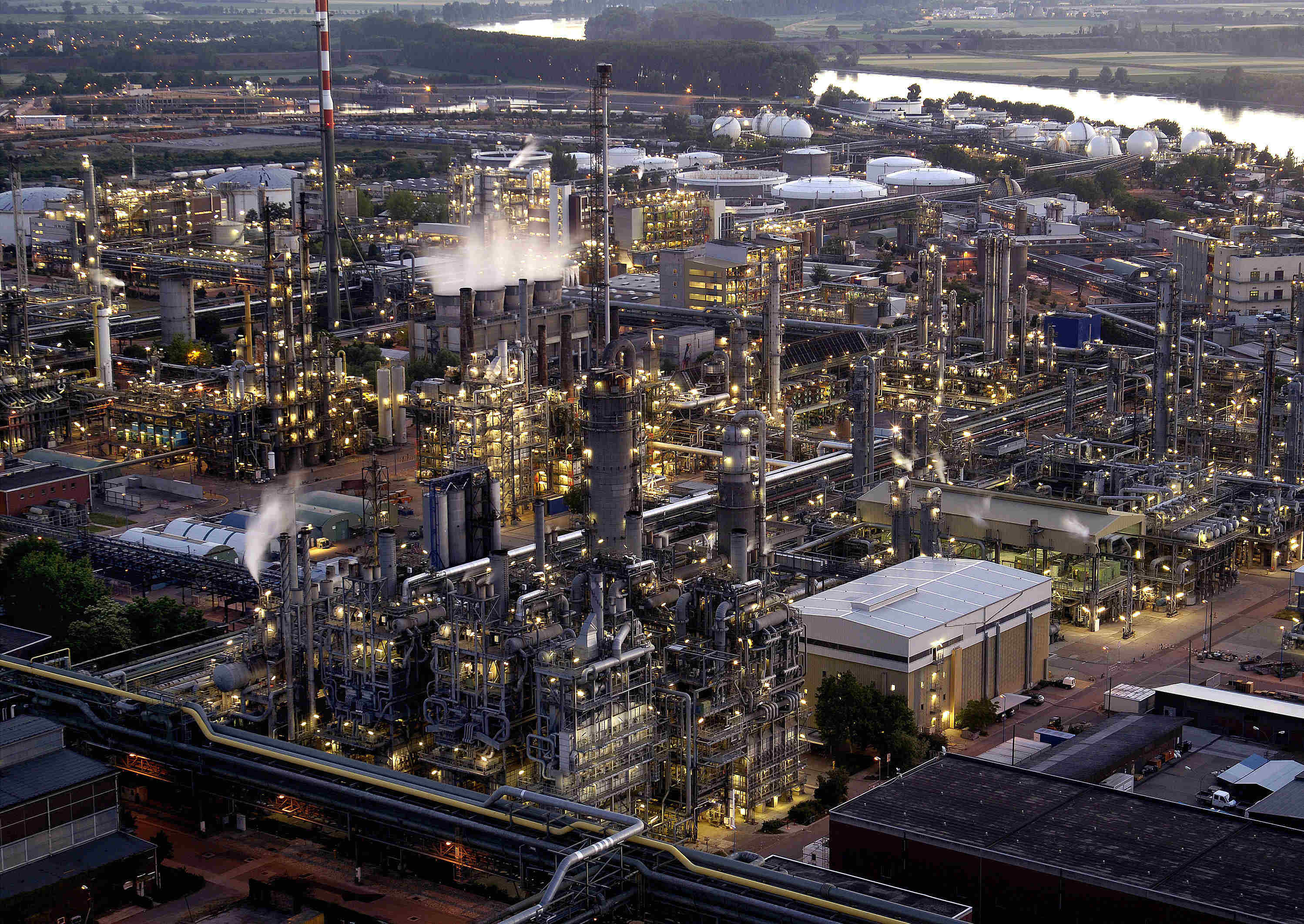
Recently, I did a project with German chemicals manufacturer BASF (wiki link). BASF is the largest chemicals manufacturer in the world, and the Ludwigshafen site pictured above is the largest chemical production complex in the world (I recommend doing a tour, it's free and very interesting).
In this blog post, I will summarize a part of the results of this project that I think could be interesting for the wider Machine Learning community. I will cut out almost all of the chemical engineering parts, as that is not my area of expertise and this blog post is directed at the ML community. A pre-print of our results is also on arxiv.
Structured ML-based plant models

The main idea of this project was to turn a "flowsheet" of a chemical plant into a structured ML model. A flowsheet is the underlying graphical representation of chemical plant simulators. Chemical plants are complex, but this complexity arises from connecting a collection of much simpler units, think "pump", "valve", "reactor", "distillation column" etc. The left part of above image is an abstraction of such a flowsheet. On the right you see what we're trying to build: we try to replace each unit with an ML model and connect the ML models in the same way as the flowsheet. Pictured here are neural networks, but any ML method would do.
The problem with cycles
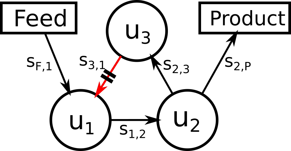
Cycles are an almost inevitable part of chemical plant design. For our ML-based plant simulation, they present a formidable challenge. There can even be nested cycles, which are particularly nasty to solve. The problem is as follows: imagine you have trained models for units u1, u2 and u3. Now you want to enter a new input into "Feed" and find out what the output and the intermediate streams may be. Propagating the information along the arrows runs into a problem already at unit u1. u1 "knows" the input from Feed, but it doesn't have information about the input coming from u3.
Many chemical plants operate in a steady-state. This means that the momentary amount of chemicals they consume and produce is always the same. We can use this to find values for the missing streams. Step 1 is to idnetify what is called a "tear stream". This can be any stream along the cycle, but often times the stream where the cycle "closes" is chosen (as indicated above). Step two is to realize that the composition of the units u1, u2 and u3 is a function, let's call it f (it is also called the "flowsheet response"), and the output of this function needs to be equal to its input: f(x) = x.
Fixed point iteration
One way to find a point where f(x) = x is to start with an initial value for the tear stream and then repeatedly apply the function to it: f(f(f(f(f(x))))). In chemical engineering, this is called the "direct substitution" method. Mathematically, this is also called a fixed point iteration. If we plot successive values of a fixed point iteration, we can represent each step in a "staircase plot", were for each step we move toward the diagonal where f(x) = x, and then go vertically towards the function:
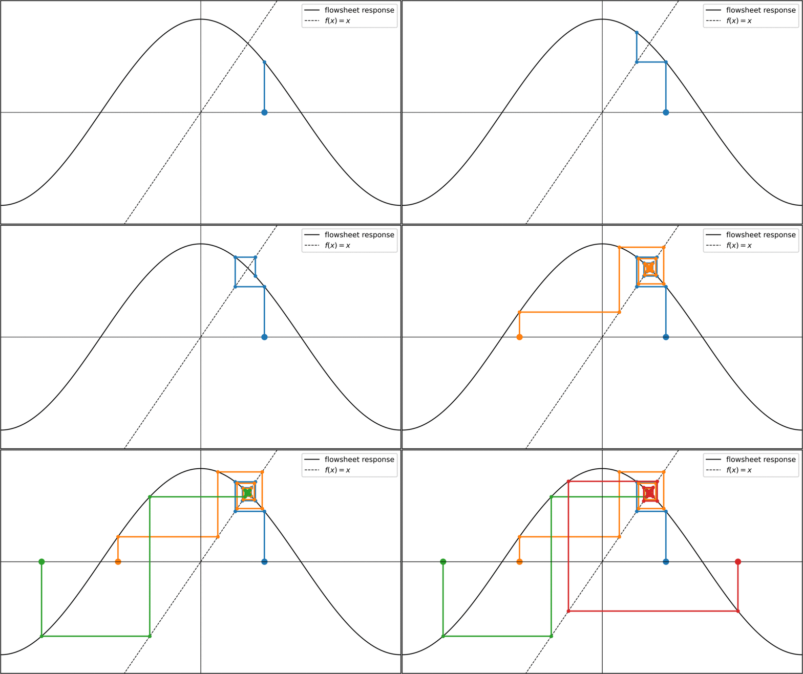
For the cosine function, any starting value converges towards the same fixed point. Of course, this is not always the case. Take a parabola for instance:
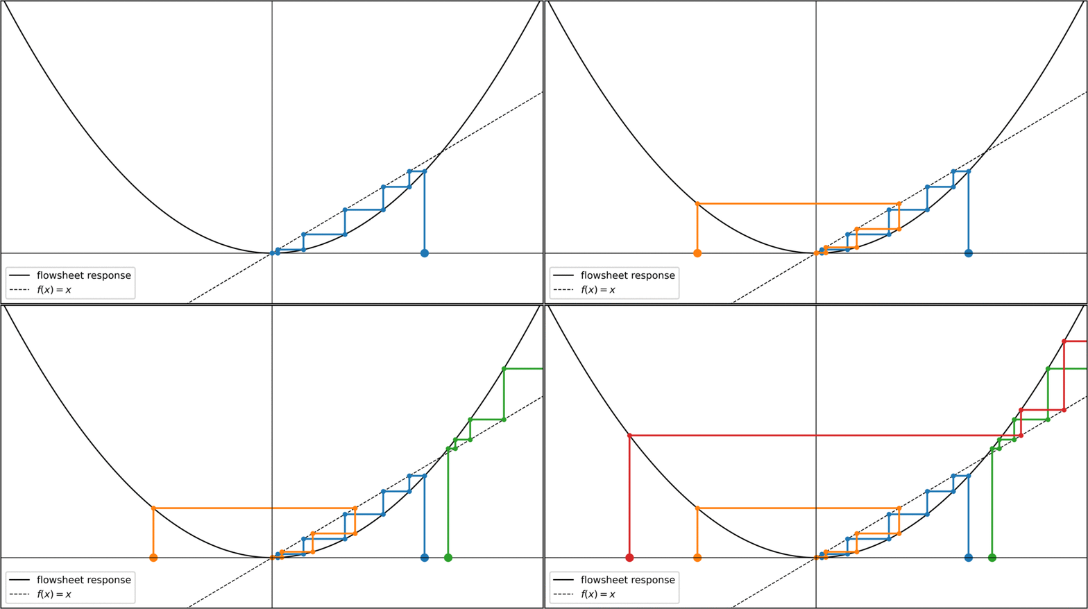
For initial values x < -1 or x > 1, the fixed-point iteration diverges towards infinity. Can we do something about this? Yes, something very simple. We can rewrite our condition f(x) = x slightly to see that f(x) - x = 0. Calling the left hand side F(x), we can say that we're looking for roots of a function F = f(x) - x. Any root-finding method can then be used to converge towards the fixed points, for instance the Newton method:
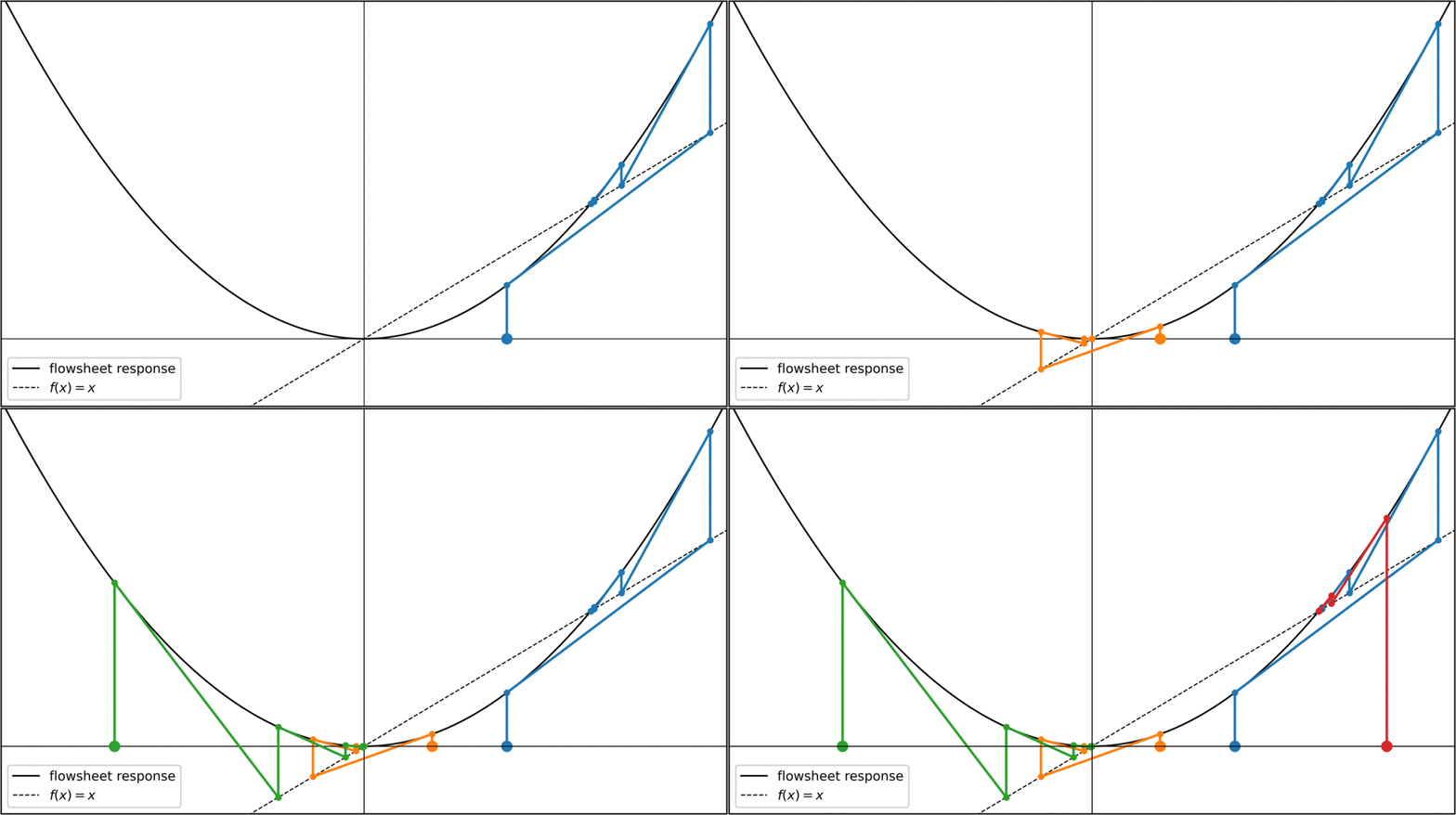
Now, for values x > 0.5, the iteration goes towards the fixed-point at x = 1. Notice how x = 1 was an unstable fixed point before, but with the Newton method it has now become a stable fixed point. Theoretically I think this should be a problem for chemical engineering problems, as we are only interested in fixed points that are stable for the original fixed point iteration. In practice, however, this doesn't seem to be a problem, at least I haven't seen it mentioned in the literature.
Fine-tuning ML models to induce stable fixed points
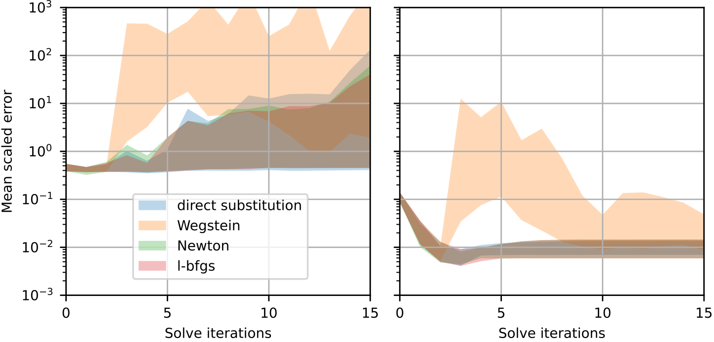
When we turned towards bigger chemical plants with and turned them into ML-based simulations, solving of the cycles did not work anymore. We tested four different solve methods, the two mentioned above (direct substitution and Newton), plus the derivative-free "Wegstein" method (an industry standard) and the BFGS algorithm. The result was always the same: What happened was that values for the tear stream often diverged towards positive or negative infinity.
After some experimentation (and a lot of debugging!), we finally found a rather simple method to fix the convergence towards the true values for the tear stream. Essentially, our innovation is training step two, in which we perform a full forward fixed-point iteration (with whichever solve method), and then use automatic differentiation to compute gradients all the way through the unrolled graph.
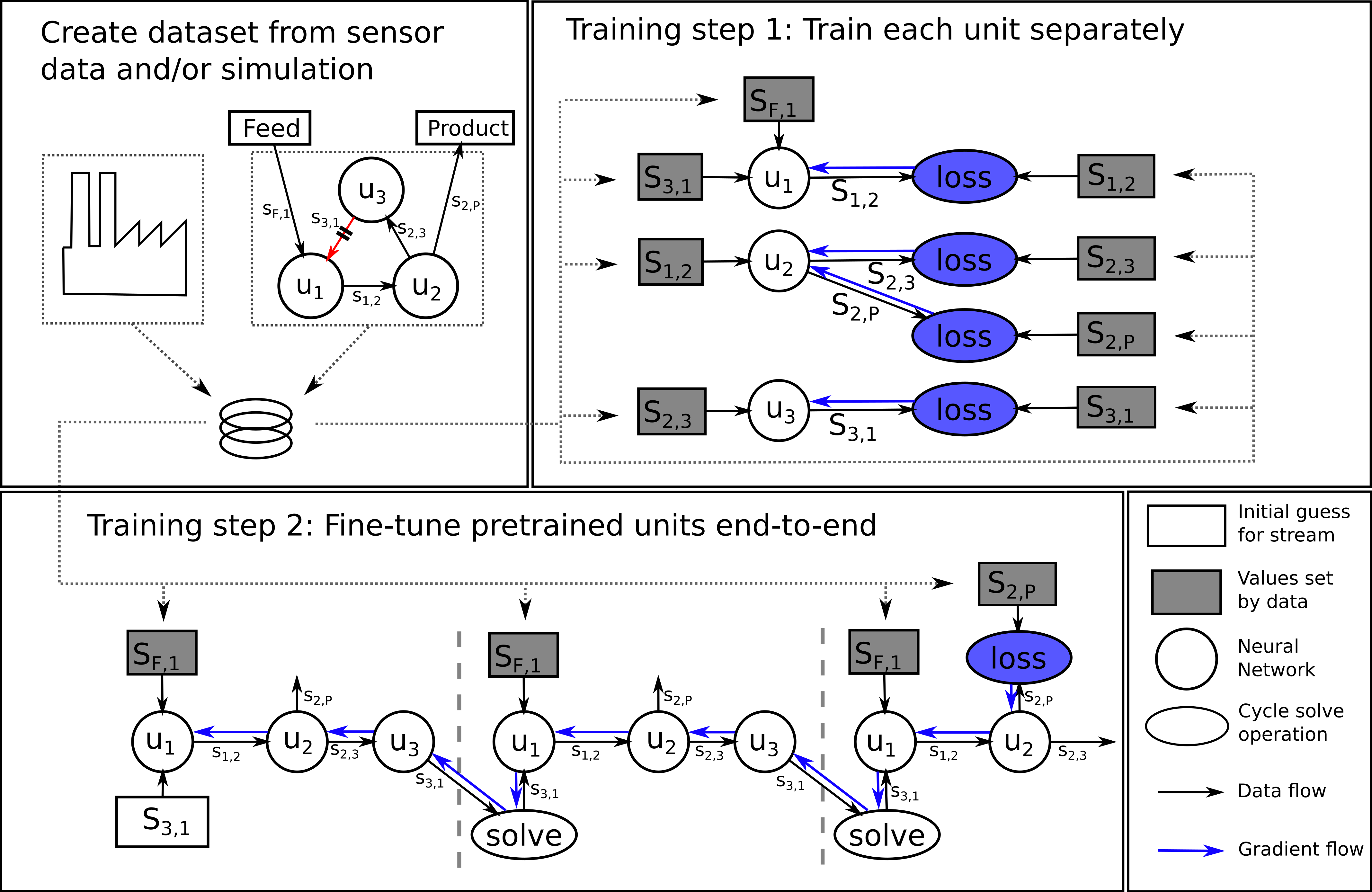
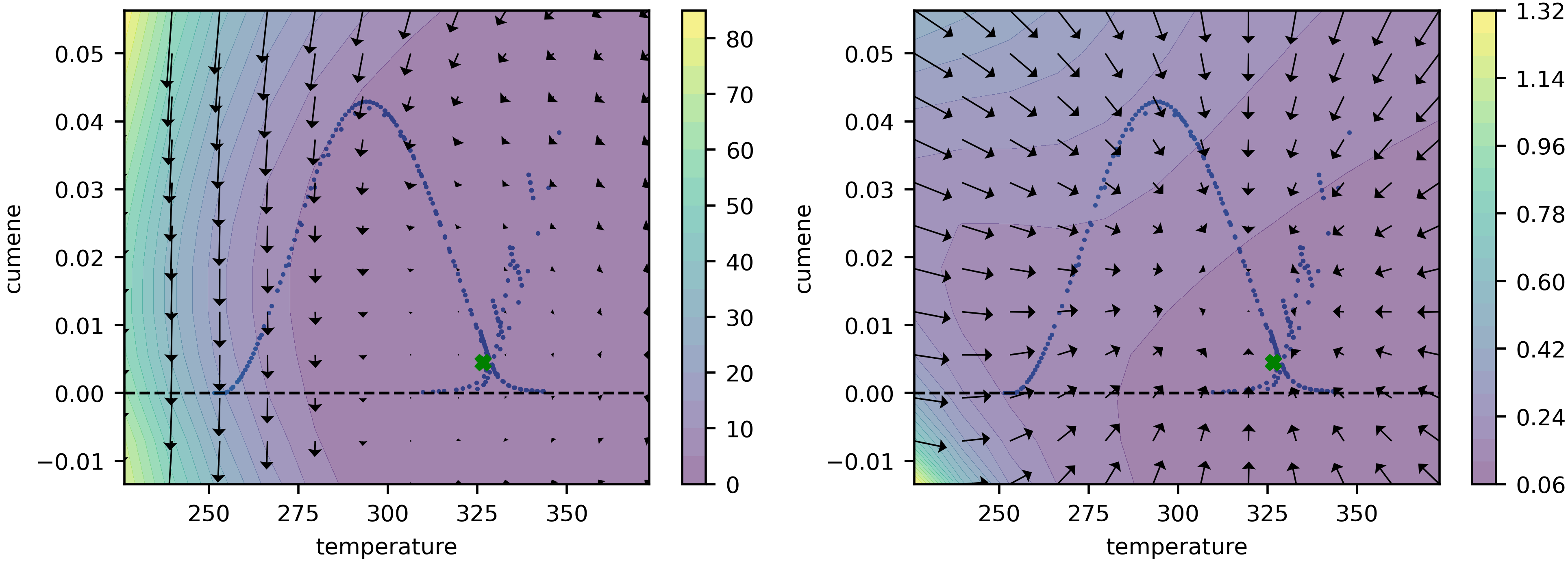
Using the gradients from training step 2, we can update the ML models u1, u2 and u3 slightly (we call it "fine-tuning"), such that their fixed points correspond to the true values. To prove that this is the case, we show a phase diagram of the fixed-point iteration before and after fine-tuning:
Similarly, we can see that the prediction error after fine-tuning is much lower (notice the log scale):
Conclusions
Fixed-point iteration towards an equilibrium point is a rather general method that has applications far beyond chemical engineering. Within Machine Learning, there is en entire emerging subfield that is occupied with this topic, started by the paper "Deep Equilibrium Models". I believe that ML-based chemical plant simulation is here to stay, because ML models have much nicer mathematical properties (compared to the chemistry-based simulation) which make them suitable for optimization. So ML models will find their place as surrogate models either on their own or in a hybrid with chemistry-based simulation.